Introduction to tidymodels
Catalina Canizares
Agenda
- What is
tidymodels - Why bother
- Example 1
- The building blocks
- Resampling with
tidymodels
Objectives
Gain an understanding of the fundamental components of the tidymodels ecosystem and appreciate the advantages of a consolidated modeling framework.
Develop the competence to independently undertake machine learning projects using R.
What is tidymodels
tidymodels is a “meta-package” for modeling and statistical analysis that shares the underlying design philosophy, grammar, and data structures of the tidyverse.
Developed by

Max Kuhn

Julia Silge
When do we get to play with tidymodels

Installing tidymodels
When loading the package, the versions and conflicts are listed:

The ecosystem

Why bother?
- They adhere to tidyverse syntax and design principles
- Automatically build tasks such as splitting, cross validation and parameter tuning
- The result of a monumental fifteen year plus effort, incorporates two hundred thirty-eight predictive models into a common framework
What is the big deal with the 238 models?
I ❤️ R but…
My 🤯 with the idiosyncratic syntax developed for different model algorithms.
More inconsistency 🤢

Dr. Raymond Balise Slides for BST 692-2022
More inconsistency 🤢
Same model, different packages
The same issue persists if you try to implement same model using alternative packages.
- Number of predictors: mtry
- Number of trees: ntree
- Number of split points: nodesize
- Number of predictors: mtry
- Number of trees: num.trees
- Number of split points: min.node.size
- Number of predictors: feature_subset_strategy
- Number of trees: num_trees
- Number of split points: min_instances_per_node
tidymodels Consistency 😎
Through the parsnip package we are provided with a time saving framework for exploring multiple models!!
Example:
# Logistic Regression
logistic_reg_glm_spec <-
  logistic_reg() %>%
  set_engine('glm') %>%
  set_mode('classification')

# Decision Tree
decision_tree_rpart_spec <-
  decision_tree(
    tree_depth = tune(),
    min_n = tune(),
    cost_complexity = tune()
  ) %>%
  set_engine("rpart") %>%
  set_mode("classification")

# Bagged MARS Model
bag_mars_earth_spec <-
  bag_mars() %>%
  set_engine('earth') %>%
  set_mode('classification')

# Naive Bayes
naive_Bayes_naivebayes_spec <-
  naive_Bayes(smoothness = tune(), Laplace = tune()) %>%
  set_engine('naivebayes') %>%
  set_mode('classification')

# Random Forest
rand_forest_randomForest_spec <-
  rand_forest(mtry = tune(), min_n = tune()) %>%
  set_engine('randomForest') %>%
  set_mode('classification')
If I haven’t convinced you yet
The real power of tidymodels is baked into the recipes package.

Binds a sequence of preprocessing steps to a training data set.
Defines the roles that the variables are to play in the design matrix.
Specifies what data cleaning needs to take place, and what feature engineering needs to happen.
Recap
- We know what
tidymodelsis - We understand its importance
- Lets starts coding…

A real, not so real example
Research Question
Are healthy behaviors, such as diet, sleep, physical activity and hours of playing video games associated with concentration in adolescents?
- Outcome: Difficulty Concentrating
- Predictors: Healthy Behaviors
Data
2019 Youth Risk Behavioral Surveillance System

Load libraries
Load the Data
EDA
Output in next slide
── Data Summary ────────────────────────
                           Values
Name                       healthyBehaviors_df
Number of rows             13677
Number of columns          20
_______________________
Column type frequency:
  character                3
  factor                   1
  numeric                  16
________________________
Group variables            None
── Variable type: character ─────────────────────────────────────────────────────────
skim_variable n_missing complete_rate min max empty n_unique whitespace
1 Sex 151 0.989 4 6 0 2 0
2 Grade 151 0.989 1 2 0 4 0
3 SexOrientation 702 0.949 8 14 0 4 0── Variable type: factor ────────────────────────────────────────────────────────────
skim_variable n_missing complete_rate ordered n_unique top_counts
1 DifficultyConcentrating 5237 0.617 FALSE 2 0: 5245, 1: 3195── Variable type: numeric ───────────────────────────────────────────────────────────
skim_variable n_missing complete_rate mean sd p0 p25 p50 p75 p100 hist
1 DrinkFruitJuice 1085 0.921 2.37 1.53 1 1 2 3 7 ▇▂▁▁▁
2 EatFruit 791 0.942 3.11 1.65 1 2 3 4 7 ▇▃▂▂▂
3 EatSalad 1779 0.870 1.97 1.23 1 1 2 2 7 ▇▁▁▁▁
4 EatPotatoes 1778 0.870 1.94 1.12 1 1 2 2 7 ▇▁▁▁▁
5 EatCarrots 1800 0.868 1.72 1.09 1 1 1 2 7 ▇▁▁▁▁
6 EatOtherVeggies 1830 0.866 2.66 1.44 1 2 2 3 7 ▇▃▂▁▁
7 DrinkSoda 2282 0.833 2.31 1.45 1 1 2 3 7 ▇▂▁▁▁
8 DrinkMilk 4188 0.694 2.64 1.64 1 1 2 4 7 ▇▂▂▁▁
9 EatBreakfast 2084 0.848 4.90 2.67 1 3 5 8 8 ▅▂▃▂▇
10 PhysicalActivity 457 0.967 4.69 2.52 1 2 5 7 8 ▇▃▆▃▇
11 HoursTV 881 0.936 2.96 1.81 1 1 3 4 7 ▇▂▃▂▂
12 HoursVideoGames 500 0.963 4.07 2.13 1 2 4 6 7 ▇▃▅▅▇
13 HoursSleep 572 0.958 3.44 1.38 1 2 4 4 7 ▇▇▇▅▂
14 SportsDrinks 4083 0.701 1.94 1.32 1 1 2 2 7 ▇▁▁▁▁
15 DrinksWater 3517 0.743 5.15 1.92 1 4 6 7 7 ▂▂▁▂▇
16 ConcussionSports 2128 0.844 1.25 0.715 1 1 1 1 5 ▇▁▁▁▁EDA
| Variable | No, N = 5,2451 | Yes, N = 3,1951 | p-value2 |
|---|---|---|---|
| Sex | <0.001 | ||
| Female | 2,328 (55%) | 1,934 (45%) | |
| Male | 2,880 (70%) | 1,229 (30%) | |
| Unknown | 37 | 32 | |
| Grade | 0.059 | ||
| 10 | 1,376 (60%) | 901 (40%) | |
| 11 | 1,232 (61%) | 775 (39%) | |
| 12 | 1,206 (64%) | 672 (36%) | |
| 9 | 1,394 (63%) | 819 (37%) | |
| Unknown | 37 | 28 | |
| SexOrientation | <0.001 | ||
| Bisexual | 236 (33%) | 473 (67%) | |
| Gay or Lesbian | 82 (42%) | 114 (58%) | |
| Heterosexual | 4,483 (67%) | 2,219 (33%) | |
| Not sure | 158 (47%) | 180 (53%) | |
| Unknown | 286 | 209 | |
Data source: MLearnYRBSS::healthyBehaviors |
|||
| 1 n (%) | |||
| 2 Pearson’s Chi-squared test | |||
EDA
Let’s explore the relationship between difficulty concentrating, diet, sleep, physical activity and hours of playing video games.

Tidymodels

Building Blocks tidymodels

1. Recipes: Preprocessing Tools
Recipes

- Every model requires a design matrix as an input.
- Design Matrix: tidy data, with one obervation per row and one predictor per column.
HOWEVER
Design matrices do not always come in the required format:
- KNN needs normalized predictors
- A linear model requires categorical predictors to be one-hot encoded
- Logistic regression needs complete data (imputation)
Recipes
healthy_recipe <-
  recipe(formula = DifficultyConcentrating ~ ., data = healthyBehaviors_df) |>
  step_zv(all_predictors()) |>
  step_impute_mode(all_nominal_predictors()) |>
  step_impute_mean(all_numeric_predictors()) |>
  step_corr(all_numeric_predictors(), threshold = 0.7) |>
  step_dummy(all_nominal_predictors())

healthy_recipe
healthy_recipe
── Recipe ───────────────────────────────────────────────────────────────────────────

── Inputs
Number of variables by role
outcome:    1
predictor: 19

── Operations
• Zero variance filter on: all_predictors()
• Mode imputation for: all_nominal_predictors()
• Mean imputation for: all_numeric_predictors()
• Correlation filter on: all_numeric_predictors()
• Dummy variables from: all_nominal_predictors()
For future models how will I know the steps?
Imperative Vs. Declarative Programming
The recipe has only sketched a blueprint of what R is supposed to do with your data. You have NOT performed any actual pre-processing yet.
Imperative Programming
- A command is entered and immediately executed
Declarative Programming
- A Command is specified and the execution code occurs at a later point in time
Baking the Recipe – Declarative Programming

This step is crucial!
You have to check your data after the recipe to make sure the transformations look alright.
# A tibble: 13,677 × 24
   DrinkFruitJuice EatFruit EatSalad EatPotatoes EatCarrots EatOtherVeggies
             <dbl>    <dbl>    <dbl>       <dbl>      <dbl>           <dbl>
 1               2        3        1           1          1               2
 2               2        7        6           5          5               6
 3               1        4        2           2          2               5
 4               2        2        1           2          2               3
 5               4        5        1           2          3               4
 6               2        1        2           1          1               2
 7               1        4        1           2          1               2
 8               4        2        2           1          2               3
 9               2        3        3           1          1               3
10               2        2        1           1          1               3
# ℹ 13,667 more rows
# ℹ 18 more variables: DrinkSoda <dbl>, DrinkMilk <dbl>, EatBreakfast <dbl>,
#   PhysicalActivity <dbl>, HoursTV <dbl>, HoursVideoGames <dbl>,
#   HoursSleep <dbl>, SportsDrinks <dbl>, DrinksWater <dbl>,
#   ConcussionSports <dbl>, DifficultyConcentrating <fct>, Sex_Male <dbl>,
#   Grade_X11 <dbl>, Grade_X12 <dbl>, Grade_X9 <dbl>,
#   SexOrientation_Gay.or.Lesbian <dbl>, SexOrientation_Heterosexual <dbl>, …
Recipes in ONE image

2. parnsip Modeling and Analysis Functions
Parsnip
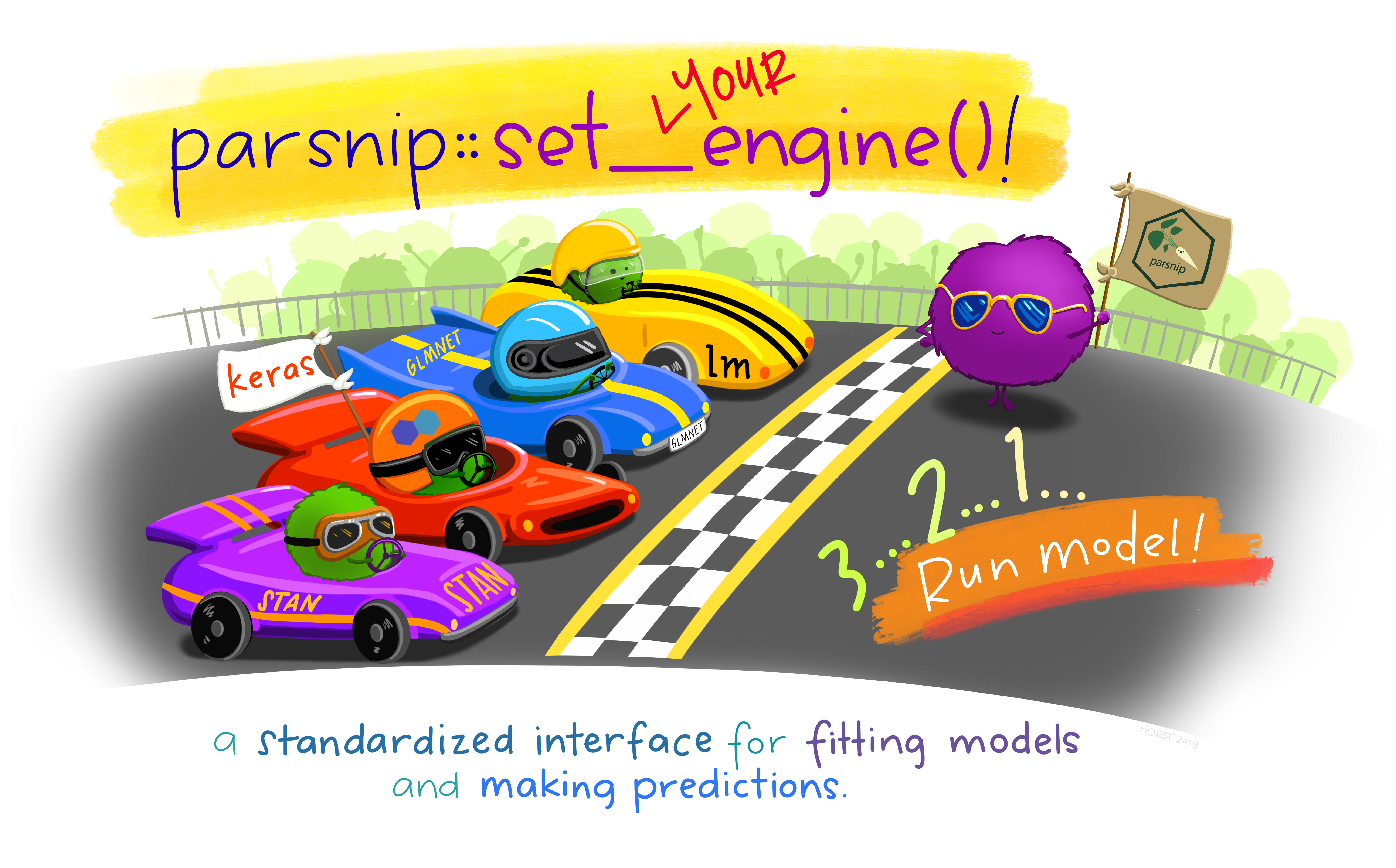
 A model specification has three individual components:
- Type: The model type that is about to be fitted (e.g., linear/logit regression, random forest or SVM).
- Mode: The mode of prediction, i.e. regression or classification.
- Engine: The computational engine implemented in
Rwhich usually corresponds to a certain modeling function (lm,glm), package (e.g.,rpart,glmnet,randomForest) or computing framework (e.g.,Stan,sparklyr).
Setting the Specifications ![]()
Logistic Regression Model Specification (classification)

Computational engine: glm
Setting the specification with help 🥹
glmnet_recipe <-
  recipe(formula = DifficultyConcentrating ~ ., data = healthyBehaviors_df) %>%
  step_zv(all_predictors()) %>%
  step_normalize(all_numeric_predictors())

glmnet_spec <-
  logistic_reg(penalty = tune(), mixture = tune()) %>%
  set_mode("classification") %>%
  set_engine("glmnet")

glmnet_workflow <-
  workflow() %>%
  add_recipe(glmnet_recipe) %>%
  add_model(glmnet_spec)

glmnet_grid <- tidyr::crossing(penalty = 10^seq(-6, -1, length.out = 20), mixture = c(0.05,
    0.2, 0.4, 0.6, 0.8, 1))

glmnet_tune <-
tune_grid(glmnet_workflow, resamples = stop("add your rsample object"), grid = glmnet_grid) parsnip in ONE image
3. Workflows
Workflows

Bundles the preprocessing recipe and model specification. It is specifically useful when you have different combinations of preprocsessing recipes and model specifications using the workflowsets package
Workflows
Workflows
══ Workflow ════════════════════════════════════════════════════════════════════
Preprocessor: Recipe
Model: logistic_reg()

── Preprocessor ────────────────────────────────────────────────────────────────
5 Recipe Steps

• step_zv()
• step_impute_mode()
• step_impute_mean()
• step_corr()
• step_dummy()

── Model ───────────────────────────────────────────────────────────────────────
Logistic Regression Model Specification (classification)

Computational engine: glm
Fit
When calling fit() on a workflow object, tidymodels performs the following steps for us:
- It fits the recipe object to the training set and produces the in-sample estimates
(prep()). - It applies the fitted recipe to the training set to process the predictors
(bake()). - It trains the specified model on the transformed set.
══ Workflow [trained] ══════════════════════════════════════════════════════════
Preprocessor: Recipe
Model: logistic_reg()

── Preprocessor ────────────────────────────────────────────────────────────────
5 Recipe Steps

• step_zv()
• step_impute_mode()
• step_impute_mean()
• step_corr()
• step_dummy()

── Model ───────────────────────────────────────────────────────────────────────

Call:  stats::glm(formula = ..y ~ ., family = stats::binomial, data = data)

Coefficients:
                  (Intercept)                DrinkFruitJuice
                     1.189158                       0.033634
                     EatFruit                       EatSalad
                    -0.033360                       0.017283
                  EatPotatoes                     EatCarrots
                    -0.011599                       0.014300
              EatOtherVeggies                      DrinkSoda
                    -0.044080                       0.095641
                    DrinkMilk                   EatBreakfast
                     0.009112                      -0.077012
             PhysicalActivity                        HoursTV
                    -0.046420                      -0.009816
              HoursVideoGames                     HoursSleep
                     0.078953                      -0.205415
                 SportsDrinks                    DrinksWater
                    -0.015897                       0.035184
             ConcussionSports                       Sex_Male
                     0.191596                      -0.584480
                    Grade_X11                      Grade_X12
                    -0.060290                      -0.229387
                     Grade_X9  SexOrientation_Gay.or.Lesbian
                    -0.021481                      -0.174600
  SexOrientation_Heterosexual        SexOrientation_Not.sure
                    -1.033922                      -0.410411

Degrees of Freedom: 8439 Total (i.e. Null);  8416 Residual
  (5237 observations deleted due to missingness)
Null Deviance:      11200
Residual Deviance: 10230    AIC: 10270
Tidy
Tidy
# A tibble: 24 × 7
   term            estimate std.error statistic p.value conf.low conf.high
   <chr>              <dbl>     <dbl>     <dbl> <chr>      <dbl>     <dbl>
 1 (Intercept)        3.28    0.157       7.57  <0.001     2.42      4.47
 2 DrinkFruitJuice    1.03    0.0176      1.91  0.056      0.999     1.07
 3 EatFruit           0.967   0.0180     -1.86  0.063      0.934     1.00
 4 EatSalad           1.02    0.0238      0.726 0.468      0.971     1.07
 5 EatPotatoes        0.988   0.0244     -0.475 0.635      0.942     1.04
 6 EatCarrots         1.01    0.0262      0.545 0.586      0.963     1.07
 7 EatOtherVeggies    0.957   0.0206     -2.14  0.032      0.919     0.996
 8 DrinkSoda          1.10    0.0182      5.26  <0.001     1.06      1.14
 9 DrinkMilk          1.01    0.0160      0.569 0.569      0.978     1.04
10 EatBreakfast       0.926   0.00954    -8.07  <0.001     0.909     0.943
# ℹ 14 more rows
glance
# A tibble: 1 × 8
  null.deviance df.null logLik    AIC    BIC deviance df.residual  nobs
          <dbl>   <int>  <dbl>  <dbl>  <dbl>    <dbl>       <int> <int>
1 11197. 8439 -5113. 10274. 10443. 10226. 8416 8440Understanding the Effect Sizes
tidy_model|>
  filter(term != "(Intercept)") |>
  ggplot(aes(reorder(term, estimate),
    y = (estimate),
    ymin = conf.low,
    ymax = conf.high
  )) +
  geom_pointrange(alpha = 0.8) +
  labs(
    y = "Odd Ratio CI",
    title = "Multiple Logistic Regression Model for \nDifficulty Concentrating",
    x = ""
  ) +
  ggeasy::easy_center_title() +
  geom_hline(yintercept = 1, linetype = "dashed") +
  coord_flip() +
  theme_minimal(base_size = 13) +
  theme(panel.grid.major = element_blank(), panel.grid.minor = element_blank()) +
  theme(legend.position = "none")
Understanding the Effect Sizes

The Prediction
# A tibble: 13,677 × 4
   DifficultyConcentrating .pred_class .pred_0 .pred_1
   <fct>                   <fct>         <dbl>   <dbl>
 1 0                       0             0.567   0.433
 2 0                       0             0.856   0.144
 3 0                       0             0.750   0.250
 4 1                       0             0.597   0.403
 5 0                       0             0.570   0.430
 6 1                       1             0.252   0.748
 7 1                       0             0.548   0.452
 8 1                       0             0.659   0.341
 9 1                       0             0.762   0.238
10 0                       0             0.761   0.239
# ℹ 13,667 more rows
Confusion Matrix
          Truth
Prediction    0    1
         0 4559 2048
         1  686 1147
A Quick Logistic Regression With Tidymodels
A Quick Logistic Regression With Tidymodels
parsnip model object


Call:  stats::glm(formula = DifficultyConcentrating ~ ., family = stats::binomial,
    data = data)

Coefficients:
                 (Intercept)                       SexMale
                   1.2966694                    -0.5731123
                     Grade11                       Grade12
                  -0.0513235                    -0.2553549
                      Grade9  SexOrientationGay or Lesbian
                  -0.0429090                    -0.1678315
  SexOrientationHeterosexual        SexOrientationNot sure
                  -1.0981269                    -0.5012433
             DrinkFruitJuice                      EatFruit
                   0.0341525                    -0.0291307
                    EatSalad                   EatPotatoes
                   0.0008994                    -0.0175496
                  EatCarrots               EatOtherVeggies
                   0.0052448                    -0.0352736
                   DrinkSoda                     DrinkMilk
                   0.1025460                     0.0194007
                EatBreakfast              PhysicalActivity
                  -0.0830040                    -0.0450063
                     HoursTV               HoursVideoGames
                  -0.0070738                     0.0705074
                  HoursSleep                  SportsDrinks
                  -0.2064308                    -0.0332756
                 DrinksWater              ConcussionSports
                   0.0332187                     0.2089819

Degrees of Freedom: 7507 Total (i.e. Null);  7484 Residual
  (6169 observations deleted due to missingness)
Null Deviance:      9948
Residual Deviance: 9044     AIC: 9092
Visualize With tidy
Visualize With tidy
# A tibble: 24 × 7
   term                  estimate std.error statistic p.value conf.low conf.high
   <chr>                    <dbl>     <dbl>     <dbl> <chr>      <dbl>     <dbl>
 1 (Intercept)              3.66     0.167      7.77  <0.001     2.64      5.08
 2 SexMale                  0.564    0.0554   -10.3   <0.001     0.506     0.628
 3 Grade11                  0.950    0.0710    -0.723 0.470      0.826     1.09
 4 Grade12                  0.775    0.0722    -3.54  <0.001     0.672     0.892
 5 Grade9                   0.958    0.0697    -0.616 0.538      0.836     1.10
 6 SexOrientationGay or…    0.845    0.180     -0.934 0.350      0.595     1.21
 7 SexOrientationHetero…    0.333    0.0914   -12.0   <0.001     0.278     0.398
 8 SexOrientationNot su…    0.606    0.147     -3.42  <0.001     0.454     0.807
 9 DrinkFruitJuice          1.03     0.0188     1.82  0.069      0.997     1.07
10 EatFruit                 0.971    0.0193    -1.51  0.131      0.935     1.01
# ℹ 14 more rows
Now, lets try splitting our data and trying different resampling methods
The Data - riskyBehaviors
Rows: 13,677
Columns: 50
$ Sex                            <chr> "Male", "Male", "Female", "Male", "Male…
$ Race                           <chr> "Multiple-Hispanic", "Multiple-Non-Hisp…
$ Age                            <int> 16, 15, 15, 15, 16, 15, 16, 15, 15, 16,…
$ Grade                          <chr> "10", "10", "10", "10", "10", "10", "10…
$ SexOrientation                 <chr> "Heterosexual", "Heterosexual", "Hetero…
$ SeatBealtUse                   <chr> "Most of the Times", "Always", "Most of…
$ DrinkingDriver                 <dbl> 1, 2, 1, 1, 1, 1, 1, 1, 5, 1, 1, 3, 1, …
$ DrivingDrinking                <dbl> 2, 2, 2, 1, 1, 1, 2, 1, 1, 2, 2, 1, 2, …
$ TextingDriving                 <dbl> 2, 2, 2, 1, 1, 1, 6, 1, 1, 8, 2, 1, 2, …
$ WeaponCarrying                 <dbl> 1, 1, 1, 1, 1, 1, 1, 1, 1, 1, 4, 1, 1, …
$ WeaponCarryingSchool           <dbl> 1, 1, 1, 1, 1, 1, 1, 1, 1, 1, 1, 1, 1, …
$ GunCarrying                    <dbl> 1, 1, 1, 1, 1, 1, 1, 1, 1, 1, 1, 1, 1, …
$ UnsafeAtSchool                 <dbl> 1, 1, 1, 1, 1, 3, 1, 1, 1, 1, 1, 1, 1, …
$ InjuredInSchool                <dbl> 1, 1, 1, 1, 1, 1, 1, 3, 1, 1, 1, 1, 1, …
$ PhysicalFight                  <dbl> 1, 1, 1, 1, 1, 1, 2, 1, 1, 3, 1, 1, 1, …
$ SchoolPhysicalFight            <dbl> 1, 1, 1, 1, 1, 1, 1, 1, 1, 1, 1, 1, 1, …
$ SexualAbuse                    <fct> 0, 0, 0, 0, 0, 0, 0, 0, 0, 0, 0, 0, 0, …
$ TimesSexualAbuse               <dbl> 1, 1, 1, 1, 1, 1, 1, 1, 1, 1, 1, 1, 1, …
$ SexualAbuseByPartner           <dbl> 2, 2, 1, 2, 1, 1, 2, 2, 2, 2, 2, 1, 1, …
$ Bullying                       <fct> 0, 1, 0, 0, 0, 1, 1, NA, 1, 0, 0, 1, 1,…
$ CyberBullying                  <fct> 0, 0, 0, 0, 0, 0, 0, NA, 1, 0, 0, 1, 0,…
$ SmokingCigarette               <fct> 0, 0, 0, 1, 0, 0, 0, 0, 0, 0, 0, 1, 1, …
$ AgeFirstCig                    <dbl> 1, 1, 1, 4, 1, 1, 1, 1, 1, 1, 1, 6, 5, …
$ DaysSmokingCigarette           <dbl> 1, 1, 1, 3, 1, 1, 1, 1, 1, 1, 1, 1, 1, …
$ CigPerDay                      <dbl> 1, 1, 1, 2, 1, 1, 1, 1, 1, 1, 1, 1, 1, …
$ Vaping                         <fct> 0, 1, 0, 1, 0, 0, 1, 1, 1, 0, 0, 1, 1, …
$ DaysVaping                     <dbl> 1, 1, 1, 7, 1, 1, 3, 1, 1, 1, 1, 7, NA,…
$ SourceVaping                   <chr> "1", "1", "1", "4", "1", "1", "4", "1",…
$ DaysSmokelessTobacco           <dbl> 1, 1, 1, 1, 1, 1, 1, 1, 1, 1, 1, 1, 1, …
$ DaysSmokingCigar               <dbl> 1, 1, 1, 1, 1, 1, 1, 1, 1, 1, 1, 1, 1, …
$ AgeFirstAlcohol                <dbl> 1, 1, 1, 5, 1, 6, 6, 1, 5, 5, 1, 1, 1, …
$ DaysAlcohol                    <dbl> 1, 1, 1, 3, 1, 2, 2, 1, 1, 2, 1, 1, 1, …
$ BingeDrinking                  <dbl> 1, 1, 1, NA, 1, 1, 1, 1, 1, 1, 1, 1, 1,…
$ LargestNumberOfDrinks          <dbl> 1, 1, 1, NA, 1, 2, 2, 1, 1, 2, 1, 1, 1,…
$ SourceAlcohol                  <chr> "1", "1", "1", "7", "1", "6", "6", "1",…
$ TimesMarihuanaUseLife          <dbl> 1, 2, 1, 7, 1, 1, 2, 1, 5, 1, 1, 4, 1, …
$ AgeFirstMarihuana              <dbl> 1, 5, 1, 4, 1, 1, 6, 1, 5, 1, 1, 6, 1, …
$ TimesMarihuanaUse30Days        <dbl> 1, 1, 1, 6, 1, 1, 1, 1, 1, 1, 1, 2, 1, …
$ TimesSyntheticMarihuanaUseLife <dbl> 1, 1, 1, 1, 1, 1, 4, 1, 1, 1, 1, 1, 1, …
$ PainMedicine                   <dbl> 1, 1, 1, 3, 1, 3, 2, 1, 3, 1, 1, 1, 1, …
$ TimesCocaine                   <dbl> 1, 1, 1, 3, 1, 1, 1, 1, 1, 1, 1, 1, 1, …
$ TimesInhalant                  <dbl> 1, 1, 1, 1, 1, 3, 1, 1, 1, 1, 1, 1, 1, …
$ TimesHeroin                    <dbl> 1, 1, 1, 1, 1, 1, 1, 1, 1, 1, 1, 1, 1, …
$ TimesMetha                     <dbl> 1, 1, 1, 1, 1, 1, 1, 1, 1, 1, 1, 1, 1, …
$ TimesEcstasy                   <dbl> 1, 1, 1, 1, 1, 1, 1, 3, 1, 1, 1, 1, 1, …
$ TimesSteroids                  <dbl> 1, 1, 1, 1, 1, 1, 1, 1, 1, 1, 1, 1, 1, …
$ TimesNeedle                    <dbl> 1, 1, 1, 1, 1, 1, 1, 1, 1, 1, 1, 1, 1, …
$ OfferedDrugsSchool             <fct> 1, 0, 0, 1, 0, 1, 1, 0, 1, 1, 0, 1, 0, …
$ HallucinogenicDrugs            <dbl> 1, 1, 1, 3, 1, 1, 1, 4, 1, 1, 1, 1, 1, …
$ MarihuanaUse                   <fct> 0, 1, 0, 1, 0, 0, 1, 0, 1, 0, 0, 1, 0, …
Task
- Predict the likelihood of and adolescent carrying a weapon to school
# Data cleaning to transform the outocme into binary and drop NAs in the outcome

riskyBehaviors_analysis <-
riskyBehaviors |>
  mutate(
    WeaponCarryingSchool = case_when(
      WeaponCarrying == 1 ~ "No",
      WeaponCarrying %in% c(2, 3, 4, 5) ~ "Yes",
      TRUE ~ NA_character_
  )) |>
  drop_na(WeaponCarryingSchool)

riskyBehaviors_analysis |>
  ggplot(aes(x = WeaponCarryingSchool )) +
  geom_bar() +
  coord_flip() +
  theme_classic()
Task

Split Training - Testing
<Training/Testing/Total>
<7908/2636/10544>
Lets Check Our Work
Resampling
# Bootstrap sampling
# A tibble: 1,000 × 2
   splits              id
   <list>              <chr>
 1 <split [7908/2953]> Bootstrap0001
 2 <split [7908/2868]> Bootstrap0002
 3 <split [7908/2927]> Bootstrap0003
 4 <split [7908/2893]> Bootstrap0004
 5 <split [7908/2910]> Bootstrap0005
 6 <split [7908/2908]> Bootstrap0006
 7 <split [7908/2932]> Bootstrap0007
 8 <split [7908/2921]> Bootstrap0008
 9 <split [7908/2904]> Bootstrap0009
10 <split [7908/2898]> Bootstrap0010
# ℹ 990 more rows# Leave-one-out cross-validation
# A tibble: 7,908 × 2
splits id
<list> <chr>
1 <split [7907/1]> Resample1
2 <split [7907/1]> Resample2
3 <split [7907/1]> Resample3
4 <split [7907/1]> Resample4
5 <split [7907/1]> Resample5
6 <split [7907/1]> Resample6
7 <split [7907/1]> Resample7
8 <split [7907/1]> Resample8
9 <split [7907/1]> Resample9
10 <split [7907/1]> Resample10
# ℹ 7,898 more rowsSummary
- Do we understand what
tidymodelsis? - Should we do the extra typing? and why?
- What are the building blocks?
- Is there a quick way to use
tidymodels? - Is it hard to create the resmpling obects?

For next time
- Introduction to LASSO
tidymodels: A complete exampledialspackagetunepackageyardstickpackage

Want to practice:
